SetFit Model 3: Fine-Tuning Deep-Learning Model for Stance Detection
Institute of Computer Science,
Brandenburgische Technische Universität Cottbus-Senftenberg
Juan-Francisco Reyes
pacoreyes@protonmail.com
Institute of Computer Science,
Brandenburgische Technische Universität Cottbus-Senftenberg
Juan-Francisco Reyes
pacoreyes@protonmail.com
### THIS PAGE WILL BE UPDATED PERMANENTLY BASED ON INTERACTIONS ON THE FORUM, RETURN OFTEN
This document delineates the process of fine-tuning a SetFit model for Stance Detection.
The "seed" model fine-tuned with the "seed" dataset represents the baseline that should be kept or improved during the bootstrapping approach that participants will follow.
Dataset 3 v1 (172 datapoints) is split into three different files:
Training Dataset: dataset_3_4_training_anonym.jsonl, 136 datapoints.
Validation Dataset: dataset_3_5_validation_anonym.jsonl, 18 datapoints.
Testing Dataset: dataset_3_6_test_anonym.jsonl, 18 datapoints.
Pool 1: dataset_3_7_unlabeled_sentences_1.jsonl, 26,844 sentences (4.5 MB).
Pool 2: dataset_3_7_unlabeled_sentences_2.jsonl, 9,496 sentences (1.8 MB).
Pool 3: dataset_3_7_unlabeled_sentences_3.jsonl, 14,847 sentences (2.6 MB). NOTE: the sentences in Pool 2 and Pool 3 have been extracted mostly from speeches and interviews, but also from news articles. The inclusion of datapoints not representative of stance in political discourse will lead to points deduction.
This is the list and structure of files delivered to complete this project:
/images (empty, here go generated plots).
/lib
/shared_data (empty, here go datasets and other data files).
paper_c_5_dl_hop_setfit.py (HOP with Optuna to find best model).
paper_c_6_dl_test_setfit.py (use test dataset to test best model).
paper_c_7_dl_inference_setfit.py (use best model to make inferences).
Step 1: use paper_c_5_dl_hop_setfit.py to create the "seed" model using the "seed" Dataset 3 (v1 or v2).
Step 2: use paper_c_6_dl_test_setfit.py to test the model and get baseline metrics.
Step 3: use paper_c_7_dl_inference_setfit.py to make inferences on unlabeled sentences (dataset_3_7_unlabeled_sentences_1.jsonl) following the bootstrapping methodology.
Step 4: follow the error analysis process, and repeat the process weekly adding new datapoints to Dataset 3, getting the highest performance possible.
We use Optuna to find the best hyperparameters in our model. Optuna is an open-source hyperparameter optimization framework designed for machine learning. It provides an efficient way to search for the best set of hyperparameters to improve the performance of a model. Optuna's design allows for the definition of a search space for hyperparameters, which combinations are explored to find the most effective one. In the provided script.
The script for hyperparameter optimization (HOP) (paper_c_5_dl_hop_setfit.py) uses the following Optuna components:
Hyperparameter Space: The function hp_space is defined with a Trial object as its argument. This function specifies the hyperparameter search space, utilizing methods like suggest_float, suggest_int, and suggest_categorical to define ranges or sets of values for different hyperparameters.
def hp_space(trial: Trial):
  return {
    "body_learning_rate": trial.suggest_float("body_learning_rate", 1e-6, 1e-3, log=True),
    "num_epochs": trial.suggest_int("num_epochs", 1, 1),
    "batch_size": trial.suggest_categorical("batch_size", [16, 32, 64]),
    "seed": trial.suggest_int("seed", 1, 40),
    "max_iter": trial.suggest_int("max_iter", 50, 300),
    "solver": trial.suggest_categorical("solver", ["newton-cg", "lbfgs", "liblinear"]),
  }
Model Initializer: model_init takes params which are provided by Optuna during the trial. It initializes the SetFitModel with these parameters.
def model_init(params):
  params = params or {}
  max_iter = params.get("max_iter", 100)
  solver = params.get("solver", "liblinear")
  params = {
    "head_params": {
      "max_iter": max_iter,
      "solver": solver,
    }
  }
  model = SetFitModel.from_pretrained(model_id, **params)
  model.to(device)
  return model
Trainer and search Method: The Trainer object from SetFit is used to conduct the hyperparameter search. The method hyperparameter_search is called on this object, which internally uses Optuna to run trials. Each trial tests a different set of hyperparameters from the defined space. The argument n_trials specifies how many trials to run, and direction indicates whether the objective is to maximize or minimize the metric.
NUM_TRIALS = 20

...

# Initialize trainer
trainer = Trainer(
    train_dataset=train_dataset,  # training dataset
    eval_dataset=validation_dataset,  # validation dataset
    model_init=model_init,  # model initialization function
)

best_run = trainer.hyperparameter_search(direction="maximize", hp_space=hp_space, n_trials=NUM_TRIALS)
Best Parameters and Model: After the search, the best set of hyperparameters is retrieved and applied to the model. This is seen in the script where best_run.hyperparameters is used to train the best version of the model and save it. Pay attention to how the trainer is modified by adding to it a callback to generate the t-SNE plots embeddings (embedding_plot_callback) and how new arguments are added to the model. The metrics shown finally are those obtained using the test dataset.
# Apply the best hyperparameters to the best model
trainer.apply_hyperparameters(best_run.hyperparameters, final_model=True)

# Initialize callbacks
embedding_plot_callback = EmbeddingPlotCallback()

# Add callbacks to trainer
trainer.callback_handler.add_callback(embedding_plot_callback)

# Add training arguments
arguments = TrainingArguments(
  eval_steps=20,
  seed=SEED
)
trainer.args = arguments

# Train best model
trainer.train()

# Evaluate best model using the test dataset
metrics = trainer.evaluate(test_dataset, "test")
print(f"\nMetrics: {metrics}")

# Save best model
trainer.model.save_pretrained("models/3")
print("\nModel saved successfully!\n")
During the hyperparameter optimization process, the output of the script shows the information of every step of the process:
Using device: MPS
Loading data from shared_data/dataset_3_4_training_anonym.jsonl...
Loaded 136 items.
Loading data from shared_data/dataset_3_5_validation_anonym.jsonl...
Loaded 18 items.
Loading data from shared_data/dataset_3_6_test_anonym.jsonl...
Loaded 18 items.

Class distribution in training dataset: Counter({0: 68, 1: 68})
Class distribution in validation dataset: Counter({0: 9, 1: 9})
Class distribution in test dataset: Counter({0: 9, 1: 9})Map: 100%|█████████████████████████████████████████████████████████████████████████████████████████████████| 136/136 [00:00<00:00, 30833.80 examples/s] [I 2024-01-25 06:04:34,052] A new study created in memory with name: no-name-63c31869-fba6-4a73-bae3-f424f10fe34e
Trial: {'body_learning_rate': 9.262057290220783e-05, 'num_epochs': 1, 'batch_size': 16, 'seed': 36, 'max_iter': 275, 'solver': 'lbfgs'}
model_head.pkl not found on HuggingFace Hub, initialising classification head with random weights. You should TRAIN this model on a downstream task to use it for predictions and inference.
***** Running training *****
  Num examples = 587
  Num epochs = 1
  Total optimization steps = 587
  Total train batch size = 16
  0%|                                                                                                                          | 0/587 [00:00<?, ?it/s]
{'embedding_loss': 0.2847, 'learning_rate': 1.5698402186814886e-06, 'epoch': 0.0}                                              | 0/587 [00:00<?, ?it/s]
{'embedding_loss': 0.0005, 'learning_rate': 7.849201093407443e-05, 'epoch': 0.09}
{'embedding_loss': 0.0001, 'learning_rate': 8.542844508215002e-05, 'epoch': 0.17}
{'embedding_loss': 0.0002, 'learning_rate': 7.665755749671368e-05, 'epoch': 0.26}
{'embedding_loss': 0.0001, 'learning_rate': 6.788666991127732e-05, 'epoch': 0.34}
{'embedding_loss': 0.0001, 'learning_rate': 5.911578232584098e-05, 'epoch': 0.43}
{'embedding_loss': 0.0, 'learning_rate': 5.0344894740404635e-05, 'epoch': 0.51}
{'embedding_loss': 0.0001, 'learning_rate': 4.157400715496829e-05, 'epoch': 0.6}
{'embedding_loss': 0.0, 'learning_rate': 3.280311956953194e-05, 'epoch': 0.68}
{'embedding_loss': 0.0, 'learning_rate': 2.4032231984095592e-05, 'epoch': 0.77}
{'embedding_loss': 0.0, 'learning_rate': 1.5261344398659244e-05, 'epoch': 0.85}
{'embedding_loss': 0.0, 'learning_rate': 6.490456813222897e-06, 'epoch': 0.94}
{'train_runtime': 196.2393, 'train_samples_per_second': 47.86, 'train_steps_per_second': 2.991, 'epoch': 1.0}
100%|████████████████████████████████████████████████████████████████████████████████████████████████████████████████| 587/587 [03:16<00:00,  2.99it/s]
***** Running evaluation *****███████████████████████████████████████████████████████████████████████████████████████| 587/587 [03:16<00:00,  2.53it/s]
[I 2024-01-25 06:07:53,688] Trial 0 finished with value: 0.9444444444444444 and parameters: {'body_learning_rate': 9.262057290220783e-05, 'num_epochs': 1, 'batch_size': 16, 'seed': 36, 'max_iter': 275, 'solver': 'lbfgs'}. Best is trial 0 with value: 0.9444444444444444.
Notice the hyperameters used to achieve that results:
{
  'body_learning_rate': 9.262057290220783e-05,
  'num_epochs': 1,
  'batch_size': 16,
  'seed': 36,
  'max_iter': 275,
  'solver': 'lbfgs'
}.Trial: {'body_learning_rate': 1.1372066559539598e-06, 'num_epochs': 1, 'batch_size': 32, 'seed': 9, 'max_iter': 297, 'solver': 'lbfgs'}
model_head.pkl not found on HuggingFace Hub, initialising classification head with random weights. You should TRAIN this model on a downstream task to use it for predictions and inference.
***** Running training *****
Num examples = 294
Num epochs = 1
Total optimization steps = 294
Total train batch size = 32
0%| | 0/294 [00:00<?, ?it/s]
{'embedding_loss': 0.2704, 'learning_rate': 3.790688853179866e-08, 'epoch': 0.0} | 0/294 [00:00<?, ?it/s]
{'embedding_loss': 0.2276, 'learning_rate': 1.0510546365635083e-06, 'epoch': 0.17}
{'embedding_loss': 0.2035, 'learning_rate': 8.356745880873796e-07, 'epoch': 0.34}
{'embedding_loss': 0.1015, 'learning_rate': 6.202945396112507e-07, 'epoch': 0.51}
{'embedding_loss': 0.1045, 'learning_rate': 4.0491449113512206e-07, 'epoch': 0.68}
{'embedding_loss': 0.0602, 'learning_rate': 1.895344426589933e-07, 'epoch': 0.85}
{'train_runtime': 180.9631, 'train_samples_per_second': 51.988, 'train_steps_per_second': 1.625, 'epoch': 1.0}
100%|████████████████████████████████████████████████████████████████████████████████████████████████████████████████| 294/294 [03:00<00:00, 1.62it/s]
***** Running evaluation *****███████████████████████████████████████████████████████████████████████████████████████| 294/294 [03:00<00:00, 2.01it/s]
[I 2024-01-25 06:20:46,434] Trial 4 finished with value: 1.0 and parameters: {'body_learning_rate': 1.1372066559539598e-06, 'num_epochs': 1, 'batch_size': 32, 'seed': 9, 'max_iter': 297, 'solver': 'lbfgs'}. Best is trial 4 with value: 1.0.
Notice the best combination of hyperparameters:
{
  'body_learning_rate': 1.1372066559539598e-06,
  'num_epochs': 1,
  'batch_size': 32,
  'seed': 9,
  'max_iter': 297,
  'solver': 'lbfgs'
}
Notice also the final message pointing out the best trial and the accuracy value:
Best is trial 4 with value: 1.0.
Trial: {'body_learning_rate': 3.321424528042531e-06, 'num_epochs': 1, 'batch_size': 32, 'seed': 11, 'max_iter': 83, 'solver': 'liblinear'}
model_head.pkl not found on HuggingFace Hub, initialising classification head with random weights. You should TRAIN this model on a downstream task to use it for predictions and inference.
***** Running training *****
  Num examples = 294
  Num epochs = 1
  Total optimization steps = 294
  Total train batch size = 32
  0%|                                                                                                                          | 0/294 [00:00<?, ?it/s]
{'embedding_loss': 0.2689, 'learning_rate': 1.1071415093475103e-07, 'epoch': 0.0}                                              | 0/294 [00:00<?, ?it/s]
{'embedding_loss': 0.1796, 'learning_rate': 3.0698014577362782e-06, 'epoch': 0.17}
{'embedding_loss': 0.0162, 'learning_rate': 2.4407437819706478e-06, 'epoch': 0.34}
{'embedding_loss': 0.0035, 'learning_rate': 1.8116861062050167e-06, 'epoch': 0.51}
{'embedding_loss': 0.0028, 'learning_rate': 1.182628430439386e-06, 'epoch': 0.68}
{'embedding_loss': 0.0022, 'learning_rate': 5.535707546737551e-07, 'epoch': 0.85}
{'train_runtime': 180.6052, 'train_samples_per_second': 52.092, 'train_steps_per_second': 1.628, 'epoch': 1.0}
100%|████████████████████████████████████████████████████████████████████████████████████████████████████████████████| 294/294 [03:00<00:00,  1.63it/s]
***** Running evaluation *****███████████████████████████████████████████████████████████████████████████████████████| 294/294 [03:00<00:00,  1.99it/s]
[I 2024-01-25 07:07:21,958] Trial 19 finished with value: 1.0 and parameters: {'body_learning_rate': 3.321424528042531e-06, 'num_epochs': 1, 'batch_size': 32, 'seed': 11, 'max_iter': 83, 'solver': 'liblinear'}. Best is trial 4 with value: 1.0.
Notice the message mentioning the best trial and the accuracy value:
Best is trial 4 with value: 1.0.
Best run: BestRun(
  run_id='4',
  objective=1.0,
  hyperparameters={
    'body_learning_rate': 1.1372066559539598e-06,
    'num_epochs': 1,
    'batch_size': 32,
    'seed': 9,
    'max_iter': 297,
    'solver': 'lbfgs
  },
  backend=<optuna.study.study.Study object at 0x2be623f10>
)Using `evaluation_strategy="steps"` as `eval_steps` is defined.
***** Running training *****
Num examples = 587
Num epochs = 1
Total optimization steps = 587
Total train batch size = 16
0%| | 0/587 [00:00<?, ?it/s]
{'embedding_loss': 0.2892, 'learning_rate': 3.3898305084745766e-07, 'epoch': 0.0} | 0/587 [00:00<?, ?it/s]
{'eval_embedding_loss': 0.2038, 'learning_rate': 6.779661016949153e-06, 'epoch': 0.03}
huggingface/tokenizers: The current process just got forked, after parallelism has already been used. Disabling parallelism to avoid deadlocks...9it/s]
To disable this warning, you can either:
- Avoid using `tokenizers` before the fork if possible
- Explicitly set the environment variable TOKENIZERS_PARALLELISM=(true | false)
{'eval_embedding_loss': 0.0841, 'learning_rate': 1.3559322033898305e-05, 'epoch': 0.07}
{'embedding_loss': 0.0103, 'learning_rate': 1.694915254237288e-05, 'epoch': 0.09}
{'eval_embedding_loss': 0.0125, 'learning_rate': 1.996212121212121e-05, 'epoch': 0.1}
{'eval_embedding_loss': 0.0128, 'learning_rate': 1.9204545454545454e-05, 'epoch': 0.14}
{'embedding_loss': 0.0002, 'learning_rate': 1.84469696969697e-05, 'epoch': 0.17}
{'eval_embedding_loss': 0.0027, 'learning_rate': 1.84469696969697e-05, 'epoch': 0.17}
{'eval_embedding_loss': 0.0017, 'learning_rate': 1.7689393939393943e-05, 'epoch': 0.2}
{'eval_embedding_loss': 0.0023, 'learning_rate': 1.6931818181818182e-05, 'epoch': 0.24}
{'embedding_loss': 0.0002, 'learning_rate': 1.6553030303030304e-05, 'epoch': 0.26}
{'eval_embedding_loss': 0.0034, 'learning_rate': 1.6174242424242425e-05, 'epoch': 0.27}
{'eval_embedding_loss': 0.0038, 'learning_rate': 1.5416666666666668e-05, 'epoch': 0.31}
{'embedding_loss': 0.0002, 'learning_rate': 1.465909090909091e-05, 'epoch': 0.34}
{'eval_embedding_loss': 0.0034, 'learning_rate': 1.465909090909091e-05, 'epoch': 0.34}
{'eval_embedding_loss': 0.0048, 'learning_rate': 1.3901515151515153e-05, 'epoch': 0.37}
{'eval_embedding_loss': 0.0035, 'learning_rate': 1.3143939393939396e-05, 'epoch': 0.41}
{'embedding_loss': 0.0002, 'learning_rate': 1.2765151515151517e-05, 'epoch': 0.43}
{'eval_embedding_loss': 0.0042, 'learning_rate': 1.2386363636363637e-05, 'epoch': 0.44}
{'eval_embedding_loss': 0.006, 'learning_rate': 1.162878787878788e-05, 'epoch': 0.48}
{'embedding_loss': 0.0002, 'learning_rate': 1.0871212121212122e-05, 'epoch': 0.51}
{'eval_embedding_loss': 0.0042, 'learning_rate': 1.0871212121212122e-05, 'epoch': 0.51}
{'eval_embedding_loss': 0.0052, 'learning_rate': 1.0113636363636365e-05, 'epoch': 0.55}
{'eval_embedding_loss': 0.0066, 'learning_rate': 9.356060606060606e-06, 'epoch': 0.58}
{'embedding_loss': 0.0002, 'learning_rate': 8.977272727272727e-06, 'epoch': 0.6}
{'eval_embedding_loss': 0.0069, 'learning_rate': 8.59848484848485e-06, 'epoch': 0.61}
{'eval_embedding_loss': 0.0047, 'learning_rate': 7.840909090909091e-06, 'epoch': 0.65}
{'embedding_loss': 0.0001, 'learning_rate': 7.083333333333335e-06, 'epoch': 0.68}
{'eval_embedding_loss': 0.0067, 'learning_rate': 7.083333333333335e-06, 'epoch': 0.68}
{'eval_embedding_loss': 0.0048, 'learning_rate': 6.3257575757575765e-06, 'epoch': 0.72}
{'eval_embedding_loss': 0.0053, 'learning_rate': 5.568181818181818e-06, 'epoch': 0.75}
{'embedding_loss': 0.0001, 'learning_rate': 5.18939393939394e-06, 'epoch': 0.77}
{'eval_embedding_loss': 0.0073, 'learning_rate': 4.810606060606061e-06, 'epoch': 0.78}
{'eval_embedding_loss': 0.005, 'learning_rate': 4.053030303030303e-06, 'epoch': 0.82}
{'embedding_loss': 0.0001, 'learning_rate': 3.2954545454545456e-06, 'epoch': 0.85}
{'eval_embedding_loss': 0.0061, 'learning_rate': 3.2954545454545456e-06, 'epoch': 0.85}
{'eval_embedding_loss': 0.0073, 'learning_rate': 2.537878787878788e-06, 'epoch': 0.89}
{'eval_embedding_loss': 0.0079, 'learning_rate': 1.7803030303030306e-06, 'epoch': 0.92}
{'embedding_loss': 0.0001, 'learning_rate': 1.4015151515151515e-06, 'epoch': 0.94}
{'eval_embedding_loss': 0.0052, 'learning_rate': 1.0227272727272729e-06, 'epoch': 0.95}
{'eval_embedding_loss': 0.0072, 'learning_rate': 2.651515151515152e-07, 'epoch': 0.99}
{'train_runtime': 269.0917, 'train_samples_per_second': 34.903, 'train_steps_per_second': 2.181, 'epoch': 1.0}
100%|████████████████████████████████████████████████████████████████████████████████████████████████████████████████| 587/587 [04:29<00:00, 2.18it/s]
***** Running evaluation *****███████████████████████████████████████████████████████████████████████████████████████| 587/587 [04:29<00:00, 2.60it/s]
Metrics: {'accuracy': 0.9444444444444444}
Model saved successfully!The t-SNE (t-distributed Stochastic Neighbor Embedding) plots provided depict the high-dimensional embeddings of your data reduced to two dimensions for visualization purposes. t-SNE is a non-linear technique for dimensionality reduction that is particularly well-suited for the visualization of high-dimensional datasets.
The visualization shows two plots:
Training Embeddings: The plot on the left labeled "Training embeddings" shows the 2D projection of the high-dimensional space where your training dataset resides. The different colors represent different classes indicate how the data is organized in this reduced space. Ideally, you want to see clear clusters with minimal overlap, which suggests that the model is learning to differentiate between the classes in the training data.
Evaluation Embeddings: The plot on the right labeled "Evaluation embeddings at step 580 of 587" shows the embeddings of the evaluation or validation dataset.
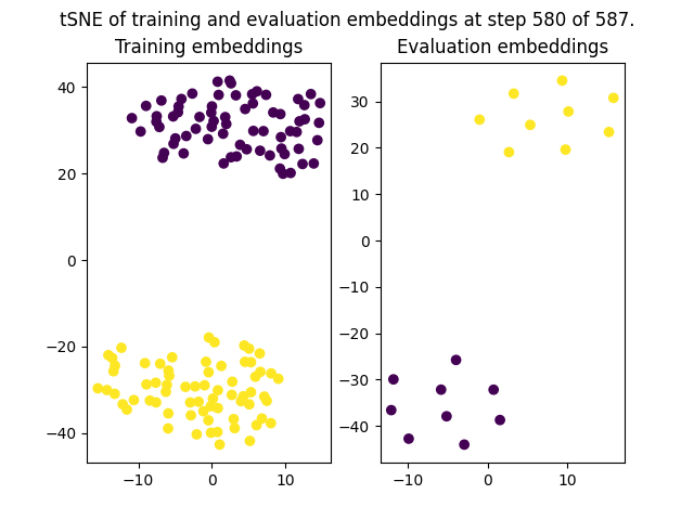
t-SNE plots are a powerful exploratory tool for understanding the feature space learned by your model. However, it is also important to complement this visual analysis with quantitative metrics.
As you see in the HOP script, a new t-SNE plots is generated every 20 steps:
# Add training arguments
arguments = TrainingArguments(
  eval_steps=20,
  seed=SEED
)
If you adjust this value, you can define the moment during the HOP process in which a new visualization is generated.
The script paper_c_7_dl_test_setfit.py is used to evaluate the pre-trained SetFit model using the test dataset, and generating more metrics and the visualization of the confusion matrix:
Loading the SetFit Model.
# Load model
model_setfit_path = "models/3"
model = SetFitModel.from_pretrained(model_setfit_path, local_files_only=True)
Setting Up Environment: First the seed (SEED) is set to ensure reproducibility. Then, the function get_device() determines the most suitable computing device (CUDA, MPS, or CPU).
# Set seed for reproducibility
set_seed(SEED)

# Move model to appropriate device
model.to(get_device())
Model Evaluation: The model is used to infer labels for the test sentences. These predictions are then compared against the true labels. The compute_metrics function calculates various performance metrics, including accuracy, precision, recall, F1 score, Area Under the Curve (AUC), and Matthews correlation coefficient (MCC). These metrics provide a comprehensive view of the model's performance. A confusion matrix is generated and plotted using plot_confusion_matrix, visually representing the model's performance.
def compute_metrics(y_pred, y_test):
  accuracy = accuracy_score(y_test, y_pred)
  precision, recall, f1, _ = precision_recall_fscore_support(y_test, y_pred, average='macro')
  auc = roc_auc_score(y_test, y_pred)
  mcc = matthews_corrcoef(y_test, y_pred)
  cm = confusion_matrix(y_test, y_pred)

  # Plot confusion matrix
  plot_confusion_matrix(y_test,
                        y_pred,
                        ["support", "oppose"],
                        "paper_c_1_dl_setfit_confusion_matrix.png",
                        "Confusion Matrix for SetFit model",
                        values_fontsize=22
                        )
  return {
    'accuracy': accuracy,
    'precision': precision,
    'recall': recall,
    'f1': f1,
    'auc': auc,
    'mcc': mcc,
    'confusion_matrix': cm
  }

...

pred_values = model.predict(sentences)

# Get labels from test dataset
true_values = [datapoint["completion"] for datapoint in test_dataset]

# Convert labels to integers
true_values = [LABEL_MAP[label] for label in true_values]

# Compute metrics
metrics = compute_metrics(pred_values, true_values)

# Create dataframe for confusion matrix
df_cm = pd.DataFrame(metrics['confusion_matrix'], index=class_names, columns=class_names)

# Print metrics
print(f"\nModel: Setfit ({model_id})\n")
print(f"- Accuracy: {metrics['accuracy']:.3f}")
print(f"- Precision: {metrics['precision']:.3f}")
print(f"- Recall: {metrics['recall']:.3f}")
print(f"- F1: {metrics['f1']:.3f}")
print(f"- AUC: {metrics['auc']:.3f}")
print(f"- MCC: {metrics['mcc']:.3f}")
print("- Confusion Matrix:")
print(df_cm)
print("\n")Model: Setfit (sentence-transformers/paraphrase-mpnet-base-v2)
- Accuracy: 0.944
- Precision: 0.950
- Recall: 0.944
- F1: 0.944
- AUC: 0.944
- MCC: 0.894
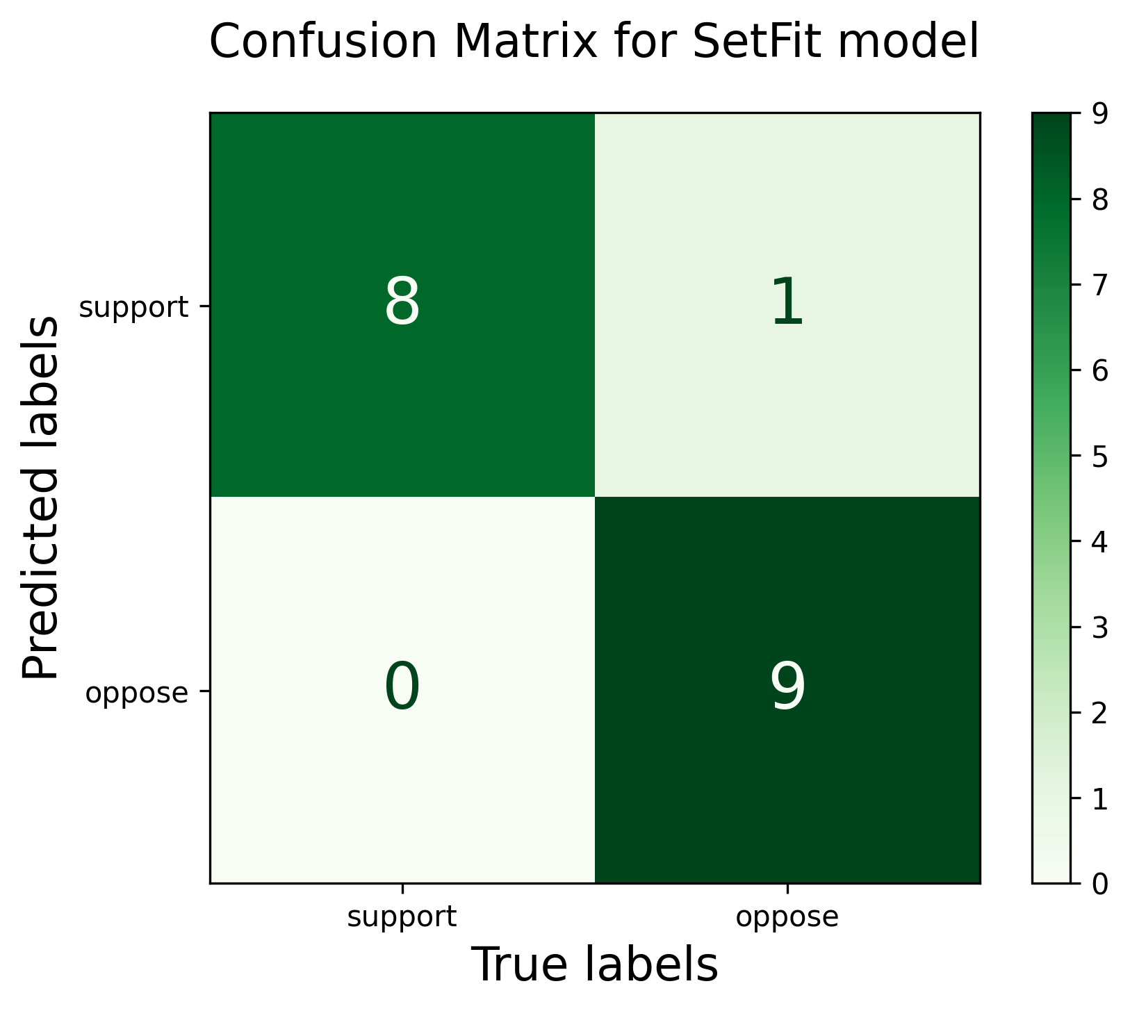
- Confusion Matrix:
support oppose
support 8 1
oppose 0 9
The confusion matrix of the SetFit model generated using the test dataset:
In NLP models optimization, while "prediction" refers specifically to the output generated by a model for given input, "inference" is the broader process of using a trained model to obtain these predictions, including data preprocessing, the actual computation through the model, and postprocessing of the results.
The code in the script paper_c_8_dl_inference_setfit.py uses the saved model to make inferences, by processing each sentence and predicting the probabilities of each class ("support" or "oppose"). The script iterates over the predicted probabilities, applies thresholds, and determines the final predicted class for each sentence. This part of the code is where the raw output from the model (probabilities) is interpreted into meaningful class labels.
# Make predictions using the model
predictions = model.predict_proba(sentences)

# Move predictions to CPU
if predictions.is_cuda:
    predictions = predictions.cpu()

# Convert predictions to list
predictions_list = predictions.numpy().tolist()

# Filter predictions by class and generate inference
for idx, p in enumerate(predictions_list):
  pred_class = None
  pred_score = 0
  if p[0] > p[1] and p[0] > 0.9945:
    pred_class = "support"
    pred_score = p[0]
  elif p[0] < p[1] and p[1] > 0.9948:
    pred_class = "oppose"
    pred_score = p[1]
  else:
    pred_class = "undefined"
  if pred_class in ["oppose", "support"]:
    print(sentences[idx])
    print(pred_class)
    print(pred_score)
print("-------")Hyperparameter Optimization using Optuna and Setfit, official SetFit documentation.