BERT Model 2: Fine-Tuning Deep-Learning Model for Passage Boundary Detection
Institute of Computer Science,
Brandenburgische Technische Universität Cottbus-Senftenberg
Juan-Francisco Reyes
pacoreyes@protonmail.com
Institute of Computer Science,
Brandenburgische Technische Universität Cottbus-Senftenberg
Juan-Francisco Reyes
pacoreyes@protonmail.com
### THIS PAGE WILL BE UPDATED PERMANENTLY BASED ON INTERACTIONS ON THE FORUM, RETURN OFTEN
This document delineates the process of preprocessing Dataset 2 and fine-tuning a BERT model for binary text classification.
Passage Boundary Detection (PBD) refers to identifying the boundaries between distinct passages or segments within a text, which is essential for tasks such as document summarization, information retrieval, and text segmentation, where understanding the structure of the text is crucial. The main challenges in PSB are:
Definition agreement: There is no universal agreement on what constitutes a "passage," as its definition can vary significantly depending on the type of text (e.g., literary texts, scientific articles, news reports, political discourse) and the specific application. This variability adds complexity to designing algorithms that can universally detect passage boundaries.
Ambiguity: Unlike sentences often delimited by clear punctuation marks, passage boundaries can be vague and unclear. Identifying where one passage ends and another begins requires understanding the linguistic features that link sentences, context, the topic, and sometimes the subtle topic shifts.
Continuity: Passages may have thematic or contextual overlaps, making determining where one topic ends and another begins is challenging. In fine-grained PBD, distinguishing these subtle changes in topic or perspective requires a sophisticated understanding and analysis of the text.
Variability: Variations in writing style, language use, and narrative techniques across different authors and text types can impact the effectiveness of PBD algorithms. Detecting boundaries in more stylistically complex or linguistically diverse texts can be particularly challenging.
Advanced NLP: Effective fine-grained PBD often requires advanced NLP techniques to understand nuanced language patterns and contextual cues. However, overall, these techniques require mainly well-annotated datasets for training.
Linguistic analysis: Understanding coherence (logical flow and connection between ideas) and cohesion (the grammatical and lexical linking within a text) is vital for effective PBD, allowing the model to process the text at a surface level and understand deeper linguistic and semantic structures.
This approach focuses on analyzing and annotating pairs of sentences to determine how they relate to each other in terms of continuity and coherence. This process is fundamental in understanding the flow of ideas and logical progression in a text.
Typically, the annotation schema includes binary labels like "Same Topic" and "Topic Change". Annotators review pairs of sentences and assign one of these labels based on the thematic continuity or discontinuity. We will use the labels "continue" and "not_continue".
Example:
[not_continue] And I want to thank Mike. Today, it's a true honor to be the first President of the United States to host a meeting at the United Nations on religious freedom.
[continue] Today, it's a true honor to be the first President of the United States to host a meeting at the United Nations on religious freedom. And an honor it is. It's long overdue.
[continue] And an honor it is. It's long overdue. And I was shocked when I was given that statistic that I would be the first.
The core idea is to analyze pairs of adjacent sentences and label them based on whether they continue the same topic or start a new one. This binary classification (same topic vs. new topic) helps identify the points where the subject matter shifts, thereby detecting topic boundaries.
In this project, the annotation will be made automatically from the annotated passages from Dataset 2.
This is the list of provided files:
build_dataset2_baseline.py: Script to convert annotated data into dataset 2 for the pair sentence labelling approach.
bert_model_2_training.py: Script to fine-tune a BERT model for sentence boundary detection using the pair sentence labelling approach.
In classical machine learning models, feature engineering is a critical step involving selecting manually and transforming raw data into a set of features that the model can understand and process effectively. In contrast, Transformer models, including BERT, are designed to automatically learn feature representations from raw text data through multiple layers of self-attention and feedforward neural networks. This process allows the model to learn complex representations of the input text without explicit manual intervention in the feature extraction process.
While fine-tuning BERT models does not entail manually selecting or creating features, it involves selecting appropriate datasets that are representative of the task at hand. For NLP projects, this involves understanding linguistic structures and features in the classification challenge. The diversity, representation, and quantity of datapoints are crucial; thus, curating a dataset that effectively represents the problem space and contains various examples for the model to learn from is essential. Additionally, converting raw text into a format for BERT models is another critical step. This process involves tokenization (breaking text into tokens), adding special tokens (like [CLS] and [SEP]), and creating attention masks. Finally, determining appropriate hyperparameters (such as learning rate, batch size, etc.) can also be considered a part of feature engineering in this context, which involves tuning the model to fit the specific characteristics of the data and the task better.
While feature engineering in the traditional sense is not a primary concern when working with BERT and similar models, the selection and preparation of data, along with model configuration and hyperparameter tuning, play a crucial role in the fine-tuning process. These steps ensure the model learns the most relevant features from the data for the specific NLP task.
Do "feature engineering" by completing first the peer review of the dataset according to the table of reviewer/reviewed. Every improvement in the dataset will impact the overall result. For this purpose, you will follow these steps:
Complete a last review of the annotation of passages ASAP, and contact your reviewers to let them know when they may start their peer review task. You can also coordinate with your reviewer to do reviews in batches according to your progress - that requires high organization between parties. The deadline for the peer review has been extended from December 8 to December 14 at 10:00. From that point, Dataset 2 will be downloaded and the grading process for dataset building (3 points) and dataset peer review (2 points) will begin; therefore, no change should be made to the dataset afterward.
Every wrong passage found in the peer review must be flagged as "to reject" in the IIA document, and the annotator (not the reviewer) must correct the mistake or reject it. Recall that the model accuracy improves whenever a wrong passage is corrected or rejected. Follow what Mr Urrego has done by logging and rejecting wrong datapoints in Mr Shresda's annotation on the shared Google Spreadsheet.
Announce on the forum when you finish your peer-review task to let your classmates know that an improved version of Dataset 2 is available to download. Effective communication and collaborative work are crucial and will be evaluated in Project 2's individual grade. See grading schema.
In the real world, building a dataset is a collaborative project; therefore, any individual contribution to improve the dataset will impact the model's performance and, in this case, the grade of every participant. Work collaboratively!!
Notice that in this project, we are trying to capture nuanced linguistic features that define topic shifts in political discourse. Likely, the number of examples (datapoints) to fine-tune a BERT model will not be enough to get a high performance. For this reason, in this complex project, we are not going to be very ambitious with performance metrics.
Download the different versions of Dataset 2 JSONL file. Each version represents a different state of the dataset along the improvement process:
dataset2_raw_dec_11.jsonl, baseline (Dec 11).
dataset2_raw_dec_13a.jsonl (Dec 13 at 16:00).
dataset2_raw_dec_13b.jsonl (Dec 13 at 22:00).
dataset2_raw_dec_16.jsonl before grading (Dec 16).
dataset2_pair_sentences_final.jsonl after grading and corrections by the lecturer (Dec 19). This version does not need to be preprocessed using the script build_dataset2_baseline.py.
Use the script build_dataset2_baseline.py to generate the annotated dataset for the sentence pair labelling annotation approach. The text will be automatically anonymized. Adjust the name of the input dataset downloaded from the links above. After processing the dataset, a new version of your dataset with the name dataset2_pair_sentences.jsonl will be generated containing pairs of sentences.
Use the training script bert_model_2_training.py. Modify hyperparameters iteratively to achieve the highest accuracy possible of the model. Use the different versions of the dataset to see the evolution of Dataset 2 and the BERT model. Register the evolution of results for the final presentation.
Use the visualizations to evaluate the performance of the model. The confusion matrix visualization (bert_model_2_confusion_matrix.png) helps you to evaluate the performance of the model by visualizing False and True Positives and Negatives in two dimensions, "Actual" and "Predicted". The training and validation losses visualization (bert_model_2_losses.png) to follow up if your model is overfitting or underfitting [link1] [link2].
A guide for tuning hyperparameters in BERT models is available here: BERT Hyperparamters: A Guide to Fine Tune BERT models.
There is an option to ignore segments of the dataset according to the annotator. For instance, you can exclude Mr Reyes's annotations in this part of the code in this way:
if passage["metadata"]["annotator"] in ["IE-Reyes"]:
  continue
You can add someone else in the list to extend the ignore block:
if passage["metadata"]["annotator"] in ["IE-Reyes", "IE-Doe"]:
  continue
In this way, you remove segments of the dataset that, for some reason, you consider they are adding noise to the model. Always ignore Mr Reyes's datapoints as implemented in the code.
| Area | Task | Description | Point weight |
|---|---|---|---|
| Dataset | Annotation | Quality, completion of annotation:
|
3 |
| Peer review | Quality, completion of annotation in assigned dataset:
|
2 | |
| Model performance | Metrics (*) | Accuracy above 0.860 in the last iteration. | 2 |
| Confusion matrix (*) | Balance between classes and a moderated imbalance ratio (<=2:10) in the final iteration. |
1.25 | |
| Training/Validation Loss (*) | The model is neither overfitted not underfitted, according to visualizations (see readings above). A small amount of overfitting is acceptable. | 1.25 | |
| Participation | Communication on the forum and collaborative work. | 0.5 | |
| Late submission | Deducted points per day. | -0.2 | |
| Total | 10 |
(*) Each grading item in Model performance must be accomplished in conjunction with the others to get its maximal grade. For instance, if accuracy is higher than 0.860 but there is a high imbalance in the confusion matrix and the training/validation losses visualization shows overfitting, only 0.75 points will be given to the three items, according to this table:
| Case 1 | Case 2 | Case 3 |
| 1 item achieved + 2 items not achieved | 2 items achieved + 1 item not achieved | 3 items achieved |
| 0.25 x 3 = 0.75 points | 0.5 x 3 = 1.5 points | 5 points |
This baseline corresponds to dataset2_raw_dec_11.jsonl, and it includes the annotations of Ms Arias, Ms Abanda, Ms Joseph, Mr Arayan, Mr Shrestha, and Mr Urrego; it does not include the segment of Mr Asgola since, at that time, his continuation in the seminar was not confirmed. I used the ignore segment option described above located in the script build_dataset2_baseline.py to exclude his annotation progress.
The provided code has the following hyperparameter values:
Resulting metrics:
| continue | not_continue | |
| continue | 190 | 103 |
| not_continue | 120 | 168 |
| continue | Precision = 0.55 | Recall = 0.62 | F1 = 0.58 |
| not_continue | Precision = 0.56 | Recall = 0.49 | F1 = 0.52 |
Training/Validation losses:
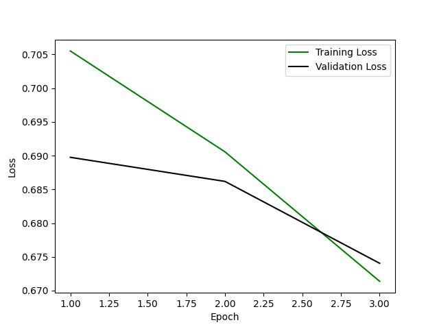
In a good fit model, both training and validation losses should decrease over time as the model learns from the data.
Training Loss: This is the error on the training split, which should decrease steadily as the model learns from the training data.
Validation Loss: This is the error on a separate dataset not seen by the model during training, used to evaluate the model's generalization capability.
If the validation loss starts to increase while the training loss continues to decrease, it may indicate overfitting, meaning the model is learning the training data too closely and not generalizing well to new, unseen data. Also, it may indicate data leakage strong regularization or that the model capacity is not fully utilized; that is, the model could be underfitting the training set.
In a confusion matrix, the acceptable level of class imbalance is not strictly defined and can vary significantly depending on the specific context and domain of the application. A balanced dataset is one where each class has approximately the same number of instances, but this is not the case in many real-world scenarios, like in this project. In practice, an imbalance ratio of 1:10 is often considered moderately imbalanced, while 1:100 or greater is highly imbalanced.Reproducibility in NLP ensures that the results of a model can be consistently achieved by different developers, across various computational environments, and at different times.
The visualization shows the training and validation losses over three epochs initially closely aligned while decreasing, indicating that the model is learning and improving its performance and not overfitting to the training data. After the middle of the second epoch, where the lines cross, the training loss decreases while the validation loss increases. This phenomenon typically indicates that the model is beginning to overfit the training data.
The model's accuracy is 0.616, indicating that approximately 61.6% of its predictions align with the ground truth. Notably, the model's precision and recall also manifest as 0.616. Precision at this level suggests that, of all instances classified positively by the model, 61.6% are indeed positive according to the actual labels. Simultaneously, the equivalent recall value indicates that the model successfully identifies 61.6% of the total true positive cases in the dataset. The confluence of accuracy, precision, and recall at the same metric value is atypical, potentially signifying a balanced distribution of classes within the dataset. Moreover, it implies a symmetrical performance by the model across both classes—neither favoring nor discriminating against any particular class.
An F1 score of 0.616 emerges from the harmonic mean of precision and recall, indicating a balanced trade-off between these metrics. Unlike an arithmetic mean, the harmonic mean penalizes extreme values more severely; thus, the F1 score is a more robust measure when dealing with imbalanced datasets. However, in this context, where precision and recall are equal, the F1 score merely mirrors these values, encapsulating the model's consistent but moderate efficacy across its predictive capabilities. While these observations suggest uniformity in the model's predictive performance, the moderate level of these metrics indicates substantial room for improvement. Specifically, enhancing the F1 score would require a focused effort to concurrently elevate both precision and recall, thereby achieving a more refined balance between the model's ability to accurately predict positive instances and its capacity to capture the majority of actual positives.
The Area Under the Receiver Operating Characteristic (AUC-ROC) curve is circa 0.7, suggesting that the model has a good separability measure, but further improvements are necessary. It can distinguish between the classes to a reasonable extent. However, the Matthews Correlation Coefficient (MCC) (0.232) is low, indicating that the model's predictions are not highly correlated with the actual values. MCC is a balanced measure even if the classes are of very different sizes. Consider MCC as a more reliable statistical rate, which produces a high score only if the prediction obtained good results in all four confusion matrix categories, proportional to both class sizes. The low score indicates that the model performs poorly in distinguishing between classes. You will see an increase in this score when the model better understands the separation between classes.
The confusion matrix shows that the model predicts "continue" better than "not_continue". However, both classes have a significant number of false positives and false negatives.
In the current state of the dataset and model, you will get different results whenever you run the script. This reproducibility issue indicates that the dataset has many misclassifications. If noise is introduced into the dataset, it will result in high variability in model performance across different runs.
While we eliminate misclassification, we will see an immediate impact in all metrics, meaning better class separations; however, we should pay close attention to MMC and the balance of classes in the confusion matrix to evaluate improvements.
Submit the following items included in a single zip file:
build_dataset2_baseline.py file.
bert_model_2_confusion_matrix.png file (5 versions, 1 per iteration/dataset version).
bert_model_2_metrics_and_hyperparameters.txt file with all metrics and hyperparameters information (5 versions, 1 per iteration/dataset version).
Create individual folders for the 5 iterations:
run1
run2
run3
run4
run5
On the session of December 19, you will present your results showing the evolution of 5 runs of your fine-tuning process using 5 versions of the raw dataset 2. In the presentations, participants will make an analysis of their results, including individual metrics, visualizations, and changes between different versions of the dataset.
The presentation includes the explanation of the early stop mechanism implemented in the code.